DOI:http://doi.org/10.65613/741750
Yucen Chen 1, Zheng Li 2*
1, College of Urban and Rural Construction,
Shanxi Argricultural University,
Jinzhong 030800, China;
Email :13222620111@163.com
2* College of Urban and Rural Construction,
Shanxi Argricultural University, Jinzhong 030800, China
Email ;lizheng@sxau.edu.cn
ABSTRACT: The Shanxi section of the Yellow River Basin is both a core area of the Loess Plateau and a national energy base. It is subject to the combined pressures of an arid climate, fragmented terrain, and coal-mining disturbance. However, the ecological cooling effects of urban wetland parks (UWPs) and their underlying driving mechanisms remain unclear in this region. This study examined 181 UWPs in the Shanxi section of the Yellow River Basin. Land surface temperature (LST) was retrieved from Landsat 8/9 remote-sensing imagery. Two indices, UWP cooling intensity (UWPCI) and UWP cooling efficiency (UWPCE), were then constructed to quantify the cooling effect. Twenty natural and anthropogenic driving factors were integrated into the analysis. Random forest (RF) and SHAP methods were used to identify the dominant driving mechanisms, while Geodetector was applied to examine spatial stratified heterogeneity. The results showed that: ① The mean UWPCI was 1.85 ± 0.42 °C, and the mean UWPCE was 0.31 ± 0.09. Spatially, high values were clustered in the central urban agglomeration, whereas low values were scattered across the western gully region. ② For UWPCI, the dominant drivers were internal water ratio (Wat_in, 32.7%), gully density (GD, 18.9%), and external impervious surface ratio (Imp_out, 12.4%). For UWPCE, park area (PA, 28.3%), coal-mining disturbance intensity (CMDI, 22.1%), and park shape index (PSI, 11.6%) were the leading factors. ③ Significant threshold effects were also detected. The marginal cooling benefit decreased when Wat_in exceeded 65%. UWPCI declined by approximately 40% when GD exceeded 2.5 km/km². UWPCE tended to become ineffective when CMDI was greater than 0.6. ④ Subregional differences were evident. In the western gully region, GD and CMDI jointly constrained the cooling effect, with an interaction contribution of 142.6%. In the central urban agglomeration, Wat_in and Imp_out were dominant. In the southern valley region, PA and Wat_in showed a coordinated optimization pattern. This study reveals the distinctive driving mechanisms of UWP cooling effects in coal-mining areas of the Loess Plateau. It proposes a differentiated optimization strategy based on zoning-based classification, threshold-based regulation, and mine–wetland coordination. The findings provide scientific support for ecological restoration and territorial spatial planning in arid and semi-arid regions.
Keywords: urban wetland park; cooling effect; driving mechanism; random forest; SHAP; Shanxi section of the Yellow River Basin; Loess Plateau; coal-mining disturbance
1 Introduction
The Shanxi section of the Yellow River Basin extends for 965 km along the middle reaches of the Yellow River. It covers 11 prefecture-level cities in Shanxi Province, with a total area of 156,000 km², accounting for 82.3% of the province’s land area. This region is a core component of the Loess Plateau and a strategic area for national energy security. It has a typical arid and semi-arid climate, with annual precipitation of 400–600 mm. Its terrain is highly fragmented, with a gully density of 1.5–3.0 km/km². Coal-mining intensity is also high, and annual coal production accounts for approximately 25% of China’s total output. Over the past 50 years, the combined effects of global warming and urbanization have increased the frequency of extreme heat events in the Shanxi section. The urbanization rate rose from 45.1% in 2010 to 62.3% in 2023. Meanwhile, the number of annual high-temperature days (the days with maximum temperature ≥35 ℃) has increased at a rate of 2.3 days per decade. These changes have posed serious threats to residents’ health, food security, and energy consumption.
Urban wetland parks (UWPs) are a key component of blue–green infrastructure[1–3,6]. They provide ecological cooling through the combined effects of water-body evaporation and vegetation transpiration[2–4,11,12]. Their cooling cost is only one-fifth to one-third of that of artificial cooling facilities, which makes them particularly valuable in arid and semi-arid regions[5]. However, UWPs in the Shanxi section of the Yellow River Basin face multiple constraints. Water scarcity limits the expansion of wetland area. Coal mining causes surface disturbance and degrades wetland ecological functions. The fragmented terrain of the Loess Plateau further restricts the diffusion of cooling effects. Shanxi is currently advancing national strategies related to ecological protection and high-quality development in the Yellow River Basin, as well as ecological restoration in coal-mining areas. Against this background, clarifying the cooling mechanisms and optimized spatial layout of UWPs in this region is essential for balancing ecological protection and economic development.
Existing studies on wetland cooling have mainly focused on national-scale assessments or humid regions[8]. Targeted evidence from the Shanxi section of the Yellow River Basin remains limited. First, regional specificity has often been overlooked. Previous studies have rarely examined how the combined effects of Loess Plateau terrain, coal-mining disturbance, and an arid climate regulate UWP cooling effects. Second, the driving-factor system remains incomplete. Key environmental factors in Shanxi, such as coal-mining disturbance and gully density, have not been adequately incorporated. Third, spatial heterogeneity has received insufficient attention. The western gully region, central urban agglomeration, and southern valley region differ markedly in both natural and socioeconomic conditions. Yet regional comparisons of cooling effects and their driving mechanisms are still lacking. Fourth, existing layout strategies are weak in practical applicability. Most recommendations have not been linked to local needs, such as ecological restoration in coal-mining areas and soil and water conservation in Shanxi. As a result, their relevance to regional policy implementation remains limited.
Based on these research gaps, this study systematically examines the cooling effects of UWPs in coal-mining areas of the Loess Plateau. It reveals the distinctive driving mechanisms shaped by the combined pressures of aridity, fragmented terrain, and coal mining, and extends the understanding of basin-scale differentiation and regional adaptation in wetland ecological effects. The study also tests the applicability of an integrated RF-SHAP-Geodetector framework in a highly heterogeneous region, thereby improving the analytical precision of ecological-effect mechanisms under complex environmental conditions. The specific objectives are to: (1) quantify the spatiotemporal differentiation of UWP cooling intensity (UWPCI) and UWP cooling efficiency (UWPCE) in the Shanxi ; (2) identify the dominant driving factors of UWP cooling effects and reveal their nonlinear relationships, threshold effects, and interaction mechanisms; (3) clarify differences in cooling effects and driving mechanisms among the western gully region, central urban agglomeration, and southern valley region; and (4) propose differentiated optimization strategies for UWP spatial layout that meet local needs in Shanxi. The proposed strategies are aligned with national priorities, including ecological restoration in coal-mining areas and ecological protection in the Yellow River Basin. They can inform urban heat island mitigation, wetland planning, and the efficient use of land resources.
2 Study area and data
2.1 Study area
The Shanxi section of the Yellow River Basin is located between 110°15′–114°33′E and 34°34′–40°43′N. It spans 11 prefecture-level cities, including Datong, Shuozhou, Xinzhou, Lüliang, Taiyuan, Yangquan, Jinzhong, Changzhi, Linfen, Jincheng, and Yuncheng (Fig. 1). As an important part of the Loess Plateau and a major national energy base, this region is shaped by the interaction between distinctive natural geographical conditions and intensive human activities. These interactions have produced a complex and heterogeneous ecological environment.
By 2026, 181 urban wetland parks (UWPs) had been identified in the Shanxi section of the Yellow River Basin[12]. Their total area reached 128.6 km². In terms of wetland type, riverine wetlands accounted for 57.3%, lacustrine wetlands for 28.1%, and artificial wetlands formed through coal-mine reclamation for 14.6%. As shown in Fig. 1, these wetland parks are mainly distributed along the Yellow River, the Fenhe River, and restored mining areas. Their spatial distribution is highly consistent with wetland and water-body land-use areas (Fig. 1c).
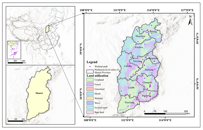
Fig. 1. Study area and spatial distribution of urban wetland parks in Shanxi Province.
Based on natural geographical characteristics, especially land-use patterns, together with socioeconomic development conditions, the Shanxi section of the Yellow River Basin can be divided into three subregions. The first is the western gully region of the Loess Plateau, which mainly includes the whole of Lüliang City and the western counties of Linfen City. This area has typical Loess Plateau landforms, with dense gullies and a gully density of 2.0-3.0 km/km². Its land use is dominated by grassland and forest land, while vegetation coverage is below 40%. Coal resources are abundant, and coal-mining activities are concentrated. The map also shows clear signs of land disturbance in this area. UWPs in this subregion are relatively scattered, and coal mining has had a substantial influence on their ecological functions and development. The second subregion is the central urban agglomeration, including Taiyuan, Jinzhong, Yangquan, and surrounding cities. This area has relatively flat and open terrain. Its land-use pattern is characterized by the interweaving of cultivated land and urban built-up areas. Urbanization has proceeded rapidly, with an urbanization rate of 65%–75% and an impervious surface ratio exceeding 50%. Fig. 1 shows that UWPs are most densely distributed in this subregion. Several wetland parks are located around Taiyuan and Jinzhong. This distribution is closely related to the increasing demand for ecological space during urban development. The third subregion is the southern Fenhe River Valley, which includes the whole of Yuncheng City and the southern counties of Linfen City. The Fenhe River runs through this area and provides relatively abundant water resources, creating milder climatic conditions. According to the land-use pattern shown in Fig. 1, cultivated land is the dominant land-use type, indicating a concentration of agricultural land. Supported by the Fenhe River, wetland resources are also relatively abundant. UWPs are therefore clustered in this subregion, and the distribution of wetlands is highly consistent with the locations of UWPs shown by the purple triangles in the map.
2.2 Data sources and preprocessing
According to the 2025 Classification List of Coal Mines in Shanxi Province issued by the Shanxi Provincial Department of Emergency Management, the coordinates of 883 coal mines were obtained. Their total production capacity was estimated at approximately 1.96 billion tons per year. Jinzhong, Lüliang, and Jincheng had the largest numbers of coal mines, with 125, 121, and 117 mines, respectively. Climate data were derived from ERA5 reanalysis data and interpolated to 0.1° raster grids using cubic spline interpolation. During the warm season from April to September, mean air temperature ranged from 14.0 to 26.2 ℃, precipitation from 281 to 641 mm, and wind speed from 11.8 to 25.3 km/h. Impervious surface data were derived from the GAIA 2020 dataset. A morphological edge-expansion algorithm was used to simulate the 2025 scenario. Urban built-up boundaries were extracted from the GUSV2021 dataset, covering 331 urban polygons in Shanxi Province with a total area of approximately 4,722.86 km².
Table 1. Data sources and preprocessing procedures.
| Data type | Specific data | Source | Time range | Preprocessing procedures |
| UWP boundary data | Vector boundaries of urban wetland parks in Shanxi Province | Amap | 2020–2026 | (1) UWPs with an area greater than 0.01 km² were selected to reflect the small wetland characteristics of Shanxi; (2) boundaries were corrected in ArcGIS to remove topological errors; (3) UWPs were classified into riverine, lacustrine, and coal-mine reclamation types. |
| Remote-sensing imagery | Landsat 8/9 OLI/TIRS and SDGSAT-1 | USGS Earth Explorer | Warm seasons from 2020 to 2025 (April–September) | (1) Images with cloud cover below 8% were selected in Google Earth Engine (GEE); (2) radiometric calibration, FLAASH atmospheric correction, and topographic correction based on the SRTM 30 m DEM were performed; (3) LST was retrieved using the single-channel algorithm; (4) warm-season mean LST was composited. |
| Land-use data | 30 m land-cover dataset for Shanxi Province | CLCD land-use dataset from Wuhan University | 2024 | (1) Internal and external vegetation, water-body, and impervious surface ratios of UWPs were extracted; (2) gully density (GD) was calculated using Fragstats 4.2; (3) all data were resampled to a 30 m resolution. |
| Coal-mining data | Coal-mining disturbance dataset for Shanxi Province | Department of Natural Resources of Shanxi Province; China Coal Research Institute | 2025 | (1) Mining-area boundaries and mining intensity were extracted; (2) coal-mining disturbance intensity (CMDI) was calculated; (3) spatial overlay analysis with UWPs was conducted. |
| Climate data | Air temperature, precipitation, and wind speed | Resource and Environmental Science Data Platform | Warm seasons from 2020 to 2024 | (1) Ordinary kriging interpolation with elevation correction was performed; (2) warm-season mean values were calculated; (3) cross-validation was conducted, with R² = 0.89. |
| Urbanization and terrain data | Urban boundaries, impervious surfaces, and DEM | GAIA dataset, SRTM 30 m DEM, and master plans of Shanxi cities | 2025 | (1) Urban built-up areas were extracted; (2) elevation and slope were calculated from the DEM; (3) the data were spatially matched with UWPs. |
To ensure the reliability and consistency of the multi-source dataset, quality control was conducted for remote-sensing, vector, thematic, and climate data. For the LST products, abnormal values were removed using the 3σ criterion, and the retrieval results were validated with 15 field observation points, yielding an RMSE of 0.92℃. For vector data, topological checking was performed to ensure spatial consistency between UWP boundaries and land-use data, and 20% of the boundaries were further verified through field surveys. For thematic variables, coal-mining disturbance intensity and gully density were normalized to the range of [0, 1] to remove dimensional differences. The interpolated climate data were compared with meteorological station records, and the relative error was less than 5%.
3 Methods
3.1 Analytical framework
This study followed an analytical framework that links data acquisition, index construction, driving-mechanism analysis, and spatial-layout optimization. The overall workflow is shown in Fig. 2 and consists of six main steps.
First, multi-source data were collected and preprocessed. UWP boundaries from 2020 to 2026 were obtained using the Amap API. After topological checking and area screening, 181 UWPs larger than 0.01 km² were retained. Landsat 8/9 OLI/TIRS imagery for the warm seasons from 2020 to 2025 was acquired from USGS Earth Explorer. Cloud-cover filtering, radiometric calibration, and atmospheric correction were completed on the GEE platform. Land-use information was extracted from the 2024 CLCD 30 m dataset to calculate vegetation, water-body, and impervious surface ratios. Coal-mine information for 2025, including 883 mines, was obtained from the Department of Natural Resources of Shanxi Province and used to calculate coal-mining disturbance intensity (CMDI). Daily meteorological data were acquired from ERA5 reanalysis data and interpolated to 0.1° raster grids. Impervious surfaces and urban boundaries were extracted from the GAIA and GUSV2021 datasets, while terrain factors were derived from the SRTM 30 m DEM.
Second, UWP cooling effects were quantified. Multi-ring buffer zones were generated outward from each UWP boundary at 50 m intervals, with a maximum distance of 1000 m. LST was retrieved using the single-channel algorithm[17–18], and the distance threshold (DT) of the cooling effect was identified for each UWP. UWP cooling intensity (UWPCI) and UWP cooling efficiency (UWPCE) were then calculated.
Third, a driving-factor system was constructed. Twenty candidate driving factors were selected from six dimensions: park geometric form, internal landscape composition, internal landscape pattern, external landscape composition, regional climate and terrain, and coal-mining disturbance. All spatial variables were resampled to a 30 m resolution and normalized when necessary.
Fourth, models were developed and interpreted. Random forest (RF) regression models were constructed to describe the nonlinear relationships between UWPCI/UWPCE and the driving factors. Hyperparameters were optimized using grid search, with n_estimators set to 500 and max_depth set to 10. The dataset was divided into training and validation sets at a ratio of 75% to 25%, and model stability was evaluated through 100 random sampling runs. SHAP was then used to quantify relative feature importance, examine partial dependence relationships, identify nonlinear and threshold effects, and assess pairwise interaction effects. Geodetector was applied to calculate q-statistics and verify spatial stratified heterogeneity.
Fifth, subregional comparisons were conducted and driving mechanisms were summarized. The study area was divided into the western gully region, central urban agglomeration, and southern valley region. ANOVA was used to test differences in cooling effects among the three subregions. Subregional RF–SHAP results and radar charts were further used to compare spatial differences in driving mechanisms. These analyses were used to summarize the driving patterns of UWP cooling effects under the combined pressures of aridity, fragmented terrain, and coal mining.
Sixth, optimized spatial-layout strategies were proposed. Based on the detected threshold effects and subregional differences, this study developed differentiated strategies centered on zoning-based classification, threshold-based regulation, and mine–wetland coordination. These strategies were aligned with ecological protection in the Yellow River Basin and ecological restoration in coal-mining areas.
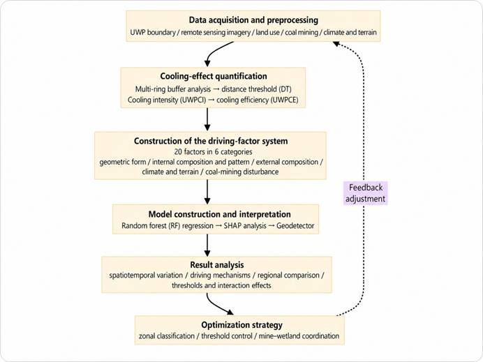
Fig. 2. Analytical framework of the study.
3.2 Calculation of cooling indices
3.2.1 Land surface temperature retrieval
Land surface temperature (LST) was retrieved from band 10 of Landsat 8/9 TIRS using the single-channel algorithm proposed by Jiménez-Muñoz et al. The algorithm is expressed as follows:
| (1) |
where Lλ is the top-of-atmosphere radiance (W·m−2·sr−1·μm−1), ε is land surface emissivity, and ψ1, ψ2, and ψ3 are atmospheric-function parameters obtained from a lookup table based on atmospheric water-vapor content. Land surface emissivity was estimated using the normalized difference vegetation index threshold method, in which fractional vegetation cover (FVC) was used to characterize vegetation conditions. γ and δ are temperature-related linearization parameters of the Planck function.
To reduce terrain-induced errors, topographic correction was performed using the SRTM 30 m DEM. The solar incidence angle was first calculated by considering slope, aspect, solar zenith angle, and solar azimuth angle. The C-correction method was then applied to correct terrain effects. Finally, annual warm-season mean LST from April to September was composited for 2020-2025 and used as the basis for analyzing UWP cooling effects.
3.2.2 Determination of the distance threshold
The distance threshold (DT) was used to define the effective spatial extent of the cooling effect for each UWP. In this study, DT was determined using multi-ring buffer analysis:
- in ArcGIS 10.8, 20 concentric buffer rings were generated outward from each UWP boundary at 50 m intervals, with a maximum radius of 1000 m. These rings were denoted as R1, R2, …, R20. R1 represented the 0–50 m ring, R2 represented the 50–100 m ring, and so forth.
- the mean LST of each buffer ring was extracted.
- a cumulative cooling-effect curve was constructed.
- the radius of the first buffer ring that satisfied the local stabilization criterion, with no smaller value occurring in the following three rings, was defined as the DT.
- for UWPs without a clear local maximum within 1000 m, accounting for 8.3% of all samples, DT was set to 1000 m. An extended search to 1500 m showed no substantial change.
This method accounts for the fragmented terrain of the Loess Plateau, where cold air can be channelized and dispersed earlier by gullies. It also avoids the inappropriate use of a fixed distance threshold derived from plain regions.
UWPCI was defined as the actual temperature reduction produced by a wetland park in relation to its surrounding environment. It was calculated as the difference between the mean LST at the distance threshold and the mean LST inside the park:
| UWPCI | (2) |
where LSTDT is the mean LST of the buffer ring at the distance threshold, and LSTin is the mean LST of all pixels within the UWP boundary. UWPCI is expressed in ℃. A higher value indicates a stronger cooling effect. For riverine wetlands, where river channels pass through the park, the area within 30 m of the water edge was defined as the internal area. This treatment was used to reduce the influence of mixed water–land pixels.
UWPCE was used to describe the cooling capacity of a wetland park per unit effective cooling area. It was calculated as the ratio of park area to the total effective cooling area:
| (3) |
where PA is the wetland park area (km²), and PCA is the park cooling area. PCA refers to the total area of all buffer rings between the UWP boundary and the distance threshold DT. Ai is the area of the i-th buffer ring (km²), and n is the number of buffer rings. UWPCE is dimensionless, with a theoretical range of (0,1). A higher value indicates a greater cooling contribution per unit cooling area and therefore higher cooling efficiency.
UWPCI and UWPCE describe different aspects of the cooling effect. UWPCI measures the magnitude of temperature reduction, or how much cooler the wetland park is than its surroundings. UWPCE measures cooling efficiency, or how much land is required to produce the cooling effect. The two indices are positively related to some extent, but they are not fully coupled. UWPs with high UWPCI and high UWPCE represent the ideal type. UWPs with high UWPCI but low UWPCE indicate strong but land-intensive cooling, which may reflect redundant water-body allocation. UWPs with low UWPCI but high UWPCE indicate small but efficient cooling units, which may be suitable for land-constrained urban areas.
3.3 Selection of driving factors
Based on the literature review and the environmental characteristics of the study area, 20 candidate driving factors were selected from six dimensions: park geometric form, internal landscape composition, internal landscape pattern, external landscape composition, regional climate and terrain, and coal-mining disturbance (Table 2). The calculation or acquisition methods for each group of factors are described below.
For park geometric form, park area (PA, km²) and park perimeter (PP, km) were obtained directly through geometric calculation in ArcGIS. The park shape index (PSI) was calculated using the formula shown below. A PSI value closer to 1 indicates a more compact park shape, whereas a higher value indicates a more elongated or fragmented shape.
| (4) |
For internal landscape composition, the 30 m CLCD land-use dataset was used to identify land-use classes within each UWP boundary. Cultivated land, forest land, grassland, and shrubland were reclassified as vegetation. Water bodies and impervious surfaces were retained as separate classes. The proportions of internal vegetation, water bodies, and impervious surfaces were then calculated. For internal water ratio (Wat_in), only perennial water surfaces were included. These water surfaces were extracted using an NDWI threshold greater than 0.2, while seasonally dry riverbeds were excluded.
For internal landscape pattern, Fragstats 4.2 was used to calculate four landscape metrics based on land-use rasters within each UWP boundary. The land-use data were reclassified into four categories: water bodies, vegetation, impervious surfaces, and bare land. Patch density (PD, number per 100 ha) was used to describe the degree of landscape fragmentation. The cohesion index (COHESION, %) measured the spatial connectivity of patches of the same class. Higher values indicate stronger spatial connectivity. The contagion index (CONTAG, %) described the dominance of large and contiguous patches. Higher values indicate that the landscape is more strongly controlled by large patches. The Shannon diversity index (SHDI) was used to represent the richness and evenness of patch types.
For external landscape composition, the area between each UWP boundary and its corresponding distance threshold (DT) was defined as the external area. The park interior was excluded from this area. External vegetation ratio (Veg_out), external water ratio (Wat_out), and external impervious surface ratio (Imp_out) were calculated within this DT-based buffer zone. Using the same DT for each UWP ensured comparability between the cooling-effect measurement and the external landscape context.
For regional climate and terrain, air temperature (Tem, ℃), precipitation (Pre, mm), and wind speed (Wind, m/s) were extracted from interpolated climate raster data. Elevation (Elev, m) and slope (Slope, °) were derived from the SRTM 30 m DEM. Gully density (GD, km/km²) was calculated within 1 km × 1 km grids. Gully lines were extracted from DEM-based hydrological analysis, and their total length was divided by grid area. The resulting grid values were then assigned to individual UWPs through bilinear interpolation.
Coal-mining disturbance intensity (CMDI) was calculated using an improved cumulative disturbance model based on data for 883 coal mines in Shanxi Province in 2025:
| (5) |
Where Ni is the number of coal mines within the 5 km buffer zone of a given UWP, Pi is the annual production capacity of the i-th coal mine, Di is the nearest distance from the UWP boundary to the coal mine, and Si is the mining-status coefficient. The coefficient was set to 1.0 for active class-A mines, 0.8 for class-B mines, 0.5 for class-C mines under rectification, 0.2 for class-D mines that had been closed but not restored, and 0 for mines with completed restoration. K is a normalization factor that scales the maximum CMDI value to 1. This model jointly considers production capacity, distance decay, and mining activity.
To remove dimensional differences, all continuous driving factors were normalized to the range of [0, 1] using min–max normalization:
| (6) |
PSI, COHESION, CONTAG, and SHDI are dimensionless indices and were not further normalized.
Table 2. Driving-factor system and descriptive statistics.
| Dimension | Factor | Code | Unit | Mean ± SD | Range | Data source |
| Geometric form | Park area | PA | km² | 0.71±0.52 | 0.11−4.83 | Corrected Amap data |
| Park perimeter | PP | km | 5.23±3.18 | 1.42−18.67 | Geometric calculation | |
| Park shape index | PSI | – | 1.68±0.47 | 1.12−4.23 | Geometric calculation | |
| Internal landscape composition | Internal vegetation ratio | Veg_in | % | 28.4±12.7 | 5.2−61.3 | CLCD 2024 |
| Internal water ratio | Wat_in | % | 48.3±18.6 | 12.5−84.2 | CLCD 2024 | |
| Internal impervious surface ratio | Imp_in | % | 15.2±8.9 | 2.1−41.6 | CLCD 2024 | |
| Internal landscape pattern | Patch density | PD | number/100 ha | 28.6±12.3 | 8.2−78.5 | Fragstats 4.2 |
| Cohesion index | COHESION | % | 86.4±7.2 | 63.8−97.2 | Fragstats 4.2 | |
| Contagion index | CONTAG | % | 54.2±11.5 | 28.6−82.3 | Fragstats 4.2 | |
| Shannon diversity index | SHDI | – | 1.18±0.34 | 0.42−1.89 | Fragstats 4.2 | |
| External landscape composition | External vegetation ratio | Veg_out | % | 31.7±15.4 | 8.6−68.3 | CLCD 2024 |
| External water ratio | Wat_out | % | 8.4±6.2 | 0.8−27.5 | CLCD 2024 | |
| External impervious surface ratio | Imp_out | % | 28.9±16.3 | 5.4−72.8 | CLCD 2024 | |
| Climate and terrain | Air temperature | Tem | ℃ | 18.6±2.4 | 14.0−26.2 | Open-Meteo/ERA5 |
| Precipitation | Pre | mm | 458±89 | 281−641 | Open-Meteo/ERA5 | |
| Wind speed | Wind | m/s | 18.7±3.2 | 11.8−25.3 | Open-Meteo/ERA5 | |
| Elevation | Elev | m | 892±346 | 186−2135 | SRTM 30 m | |
| Slope | Slope | ° | 8.6±5.8 | 0.5−28.3 | SRTM 30 m-derived product | |
| Gully density | GD | km/km² | 1.98±0.67 | 0.42−3.21 | Hydrological analysis + DEM | |
| Coal-mining disturbance | Coal-mining disturbance intensity | CMDI | – | 0.38±0.29 | 0.00−0.92 | Shanxi coal-mine list + cumulative disturbance model |
3.4 RF model construction and validation
Random forest (RF) is an ensemble learning algorithm that generates multiple decision trees through bootstrap resampling[21]. For regression tasks, the final prediction is obtained by averaging the predictions of all trees. RF has several advantages for this study. It can capture nonlinear relationships and high-order interactions among driving factors. It is also robust to outliers and noise, and provides measures of feature importance. The RF regression model can be expressed as follows:
| (7) |
where y is the predicted value, which denotes UWPCI or UWPCE in this study; Ntree is the total number of decision trees in the RF model, with the optimal value set to 500; and ht(X) is the prediction of the t-th decision tree for the input feature vector X = (x1, x2, …, xM), where M = 20 represents the total number of driving factors. The final prediction is the arithmetic mean of the predictions from all decision trees.
This study used Tree SHAP, a fast and exact SHAP algorithm specifically designed for tree-based models. Based on the trained RF models, SHAP values were calculated for each UWP sample and each feature. This produced a SHAP matrix with 181 samples, 20 features, and two dependent variables[22–23].
3.5 Importance and effect analysis
For each feature j, the mean absolute SHAP value was calculated as follows:
| (8) |
All features were ranked in descending order according to Importancej. The values were then normalized into percentages to obtain the relative importance ranking. This metric reflects the average magnitude of each feature’s contribution to model prediction. Compared with Gini-based importance, it provides a more stable interpretation of feature effects.
Partial dependence plots (PDPs) show the marginal effect of a single feature on model prediction. SHAP dependence plots further combine this marginal effect with the distribution of feature values. For a given feature xj, the SHAP dependence plot shows the scatter relationship between ϕ(j) and xj. A second feature can also be used for color coding to display potential interaction effects. In this study, the shap.dependence_plot function in the SHAP library was used to examine the nonlinear relationships and threshold effects between the core driving factors and UWPCI/UWPCE.
Thresholds were identified through three steps. ① Segmented regression was applied to the partial dependence curves to identify breakpoints. ② The Pettitt test, described in Section 3.7, was used to determine the statistical significance of the detected change points. ③ Samples were divided into below-threshold and above-threshold groups according to the identified thresholds. Independent-samples t-tests were then used to examine whether the mean differences between the two groups were significant (p < 0.05).
SHAP interaction values were defined as the part of the joint contribution of features j and k that exceeds the sum of their individual contributions. For tree-based models, the prediction can be decomposed as follows:
| (9) |
where is the SHAP interaction value between features j and k for sample i. The overall strength of the interaction effect was measured using the mean absolute SHAP interaction value:
| (10) |
3.5.4 Visualization outputs
Based on the SHAP results, three core types of figures were generated. ① SHAP summary plots were produced. In these plots, SHAP values for all samples were vertically arranged according to feature importance. The color of each point represented the original feature value, thereby showing both the direction and magnitude of feature effects. ② SHAP dependence plots were produced for the core features. These plots showed the relationship between SHAP values and original feature values. A LOESS-smoothed trend line was added to highlight nonlinear patterns and threshold effects. ③ Interaction contour plots were generated for key interaction pairs, such as Wat_in × GD. Two-dimensional grids of SHAP interaction values were plotted to identify the feature ranges where interaction effects were most evident.
3.6 Geodetector
Geodetector is a statistical method used to detect spatial stratified heterogeneity and its underlying driving factors. Its basic assumption is that if an independent variable has a strong influence on a dependent variable, the two variables should show similar spatial distributions. In this study, the factor detector module of Geodetector was used to quantify the explanatory power of each driving factor for the spatial differentiation of UWPCI.
The 181 UWPs in the study area were used as spatial sample points. UWPCI was taken as the dependent variable Y, while each driving factor was treated as an independent variable X after discretization. Geodetector requires independent variables to be categorical. Therefore, continuous driving factors, except PSI, COHESION, CONTAG, and SHDI, were discretized into five classes using the Jenks natural breaks method or the equal-interval method. Each class contained at least five samples. Sensitivity analysis showed that the q-statistic varied by less than 5% when the number of classes ranged from three to six. Five classes were therefore used in the final analysis. The q-statistic of the factor detector was calculated as follows:
| (11) |
where h = 1, 2, …, L denotes the strata of independent variable X; Nh and σh2 are the sample size and variance within stratum h, respectively; and N and σ² are the total sample size and variance of the whole study area, respectively. The q-statistic ranges from 0 to 1. A larger q value indicates stronger explanatory power of X for the spatial differentiation of Y. A value of q = 1 indicates complete control, whereas q = 0 indicates no explanatory relationship. The q-statistic follows a noncentral F distribution, and its significance was tested using 999 permutations, with p < 0.05 indicating statistical significance.
Independent Geodetector analyses were conducted for the western gully region, central urban agglomeration, and southern valley region. The q-value rankings of the dominant driving factors were then compared among the three subregions. If the coefficient of variation of the q value for a given factor exceeded 0.3 across subregions, that factor was considered to show substantial regional heterogeneity.
The interaction detector in Geodetector was also used to evaluate whether the combined effect of two factors enhanced or weakened their explanatory power for the dependent variable. The interaction types included nonlinear weakening, where q(X1 ∩ X2) < min[q(X1), q(X2)]; univariate weakening, where min[q(X1), q(X2)] < q(X1 ∩ X2) < max[q(X1), q(X2)]; bivariate enhancement, where q(X1 ∩ X2) > max[q(X1), q(X2)]; independent effect, where q(X1 ∩ X2) = q(X1) + q(X2); and nonlinear enhancement, where q(X1 ∩ X2) > q(X1) + q(X2). These results were compared with SHAP interaction values to cross-validate the identified interaction mechanisms.
3.7 Statistical analysis
One-way analysis of variance (ANOVA) was used to test whether the mean UWPCI and UWPCE values differed significantly among the three subregions: the western gully region, central urban agglomeration, and southern valley region. Before ANOVA, the assumptions of normality and homogeneity of variance were examined. Normality was tested using the Shapiro–Wilk test, and all subregions satisfied the normality assumption with p > 0.05. Homogeneity of variance was tested using Levene’s test, with p > 0.05 indicating equal variances. When the ANOVA result was significant (p < 0.05), Tukey’s honestly significant difference (HSD) test was used for post hoc pairwise comparisons. Significant differences among groups were indicated using letter labels, such as a, b, and c. Effect size was evaluated using eta-squared (η²).
Pearson correlation analysis was used to examine the linear relationship between UWPCI and UWPCE. It was also used to explore the preliminary associations between driving factors and cooling indices. For continuous variables that satisfied the normality assumption, the Pearson product–moment correlation coefficient was calculated as follows:
| (12) |
A correlation was considered significant when p < 0.05. The analysis was conducted in SPSS 26.0, and a correlation-matrix heatmap was generated to visualize the results.
The Pettitt test was used to objectively identify threshold points, or change points, along the partial dependence curves and to reduce subjectivity in threshold selection. The Pettitt test is a nonparametric method for detecting change points in continuous sequences. For a sequence of SHAP values sorted in ascending order by a given feature X, such as UWPCI values sorted by Wat_in, the test statistic is expressed as follows:
| (13) |
where sgn denotes the sign function. The p value corresponding to the Pettitt statistic was approximated as follows:
| (14) |
The location of the maximum Pettitt statistic was identified as the potential change point. When p < 0.05, the change point was considered statistically significant, and the corresponding value of X was treated as the threshold. For factors without a clear change point or with multiple potential change points, such as factors with an approximately linear relationship, the Bayesian information criterion (BIC) from segmented regression was used to determine the optimal number of segments.
Global Moran’s I was calculated for UWPCI to verify the spatial clustering pattern of UWP cooling effects. The index is expressed as follows:
| (15) |
where wij is the spatial weight matrix, defined based on inverse distance or adjacency relationships, and is the sample variance. A positive Moran’s I indicates positive spatial autocorrelation[25–26], whereas a negative value indicates spatial dispersion. A significant positive Moran’s I suggests that cooling intensity shows spatial clustering, with high-value UWPs adjacent to other high-value UWPs and low-value UWPs adjacent to other low-value UWPs. This result supports the rationale for subsequent subregional division. Global Moran’s I was calculated using GeoDa 1.18, and local indicators of spatial association (LISA) cluster maps were produced to identify local spatial association patterns.
4 Results
4.1 Spatiotemporal characteristics of UWP cooling effects in the Shanxi section
4.1.1 Overall characteristics
Based on LST retrieval from Landsat 8/9 imagery for the warm seasons from 2020 to 2025, UWPCI and UWPCE were calculated for 181 UWPs in the Shanxi section of the Yellow River Basin. The descriptive statistics are shown in Table 3.
Table 3. Overall statistics of UWP cooling effects in the Shanxi section.
| Index | Sample size | Mean ± SD | Median | Minimum | Maximum | Coefficient of variation |
| UWPCI(℃) | 181 | 1.85±0.42 | 1.81 | 0.93 | 3.21 | 0.227 |
| UWPCE | 181 | 0.31±0.09 | 0.3 | 0.14 | 0.56 | 0.29 |
For UWPCI, the regional mean was 1.85 ± 0.42 ℃, with values ranging from 0.93 to 3.21 ℃. A total of 23 UWPs had high cooling intensity, defined as UWPCI ≥ 2.5 ℃, accounting for 12.7% of all samples. These UWPs were mainly located in the Taiyuan Basin. By contrast, 31 UWPs had low cooling intensity, defined as UWPCI ≤ 1.2 ℃, accounting for 17.1% of all samples. They were mainly concentrated in the Lüliang Mountains and the coal-mining subsidence areas of northern Shanxi[29–30].
For UWPCE, the regional mean was 0.31 ± 0.09, with values ranging from 0.14 to 0.56. A total of 27 UWPs showed high cooling efficiency, defined as UWPCE ≥ 0.40, accounting for 14.9% of the samples. These parks were mainly small reclaimed coal-mining wetlands and compact wetlands in urban core areas. In contrast, 18 UWPs had low cooling efficiency, defined as UWPCE ≤ 0.22, accounting for 9.9% of the samples. Most of these parks were characterized by large area but dispersed water bodies, indicating a large but inefficient cooling pattern.
Pearson correlation analysis showed a significant positive correlation between UWPCI and UWPCE (r = 0.58, p < 0.001). This result indicates that UWPs with stronger cooling intensity in the Shanxi section usually also had higher cooling efficiency. However, the two indices were not fully linearly coupled (r² = 0.34). Two atypical combinations were observed: high-intensity but low-efficiency UWPs, such as some large lacustrine wetlands, and low-intensity but high-efficiency UWPs, such as pond clusters in mining areas.
Compared with wetland cooling effects reported in other regions of China, the mean UWPCI in the Shanxi section was approximately 23% lower than that in the Yangtze River Basin (2.4–2.6 ℃) and approximately 15% lower than that in urban wetlands of the Beijing–Tianjin–Hebei region (2.1–2.3 ℃). It was slightly higher than that in grassland wetlands in the arid region of Inner Mongolia (1.6–1.7 ℃). These comparisons suggest that the combined pressures of aridity, fragmented terrain, and coal mining constrain wetland cooling functions in the Shanxi section.
4.1.2 Spatial differentiation
The UWPCI values of the 181 UWPs were classified into five levels using the Jenks natural breaks method in ArcGIS. Their spatial distribution is shown in Fig. 3.
High-value areas, with UWPCI ≥ 2.2 ℃, were concentrated in the central urban agglomeration, mainly including Taiyuan, Jinzhong, and Yangquan. These areas formed a cool-island axis along the Fenhe River. The highest values occurred in Taiyuan Fenhe Park (2.98 ℃) and Jinzhong Xiaohe Wetland Park (2.76 ℃). In this subregion, the mean internal water ratio of UWPs reached 63.5%, and the surrounding impervious surface ratio was also high, with an average of 42%. The temperature contrast caused by the urban heat island effect amplified the apparent cooling intensity of wetland parks.
Low-value areas, with UWPCI ≤ 1.5 ℃, were mainly located in the western gully region of the Loess Plateau, including most of Lüliang and western Linfen, as well as the coal-mining subsidence areas of Datong and Shuozhou in northern Shanxi. The lowest values were observed in Lishi Wetland Park in Lüliang (1.08 ℃) and a reclaimed wetland in a mining area (1.12 ℃). These wetlands were affected by gully fragmentation and coal-mining disturbance. Cold air was difficult to diffuse horizontally, and land subsidence weakened water-body continuity.
Medium-intensity areas, with UWPCI values of 1.5–2.2 ℃, were mainly distributed in the southern Fenhe River Valley, including Yuncheng and southern Linfen. UWPCI in this area generally ranged from 1.6 to 2.1 ℃, with a relatively even spatial distribution. The cooling effect was jointly controlled by wetland area and internal water ratio.
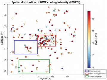
Fig. 3. Spatial distribution of UWPCI in the Shanxi section of the Yellow River Basin.
The spatial pattern of UWPCE is shown in Fig. 4. Unlike UWPCI, high UWPCE values were not limited to the central urban agglomeration. They also appeared sporadically in some reclaimed coal-mining wetlands in the western gully region. For example, one reclaimed wetland in Xing County had a UWPCE value of 0.42. These small wetlands with high internal water ratios had limited absolute cooling intensity, but their cooling contribution per unit area was high. This pattern suggests the potential value of developing micro-wetland networks in land-constrained or ecologically fragile areas.
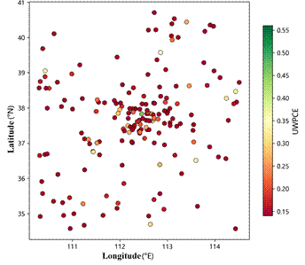
Fig. 4. Spatial distribution of UWPCE in the Shanxi section of the Yellow River Basin.
4.1.3 Temporal differentiation
From 2020 to 2025, UWPCI showed clear precipitation-controlled interannual fluctuations (Fig. 5). In 2022, an extreme drought year, warm-season precipitation was only 312 mm, 32% lower than the multi-year average. UWPCI decreased to its lowest value of 1.63 ℃. In 2024, a wet year with precipitation of 612 mm, UWPCI increased to its peak value of 2.01 ℃. The interannual range reached 0.38 ℃. This pattern indicates that wetland cooling functions in arid and semi-arid regions are highly sensitive to precipitation variability.
During the same period, UWPCE showed a smaller interannual range, varying from 0.28 to 0.34. This suggests that cooling efficiency was relatively stable and was mainly controlled by wetland morphology and land-use structure. Its response to interannual climate variability was less direct than that of cooling intensity.
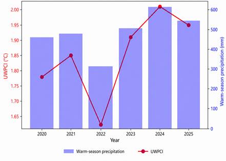
Fig. 5. Interannual variation in UWPCI and warm-season precipitation.
Monthly variation in UWPCI showed a unimodal pattern (Fig. 6). UWPCI was relatively low in April and September, with values of 1.41 ℃ and 1.52 ℃, respectively. It reached its highest levels in July and August, with values of 2.28 ℃ and 2.34 ℃, respectively. The peak months corresponded closely to the period of highest air temperature and strongest urban heat island intensity. This indicates that the cooling function of UWPs is synchronized with seasonal cooling demand.
The monthly standard deviation of UWPCI was highest in July and August, reaching 0.55 ℃. This result suggests that, during high-temperature periods, wetland-specific conditions, especially water-body scale and water supply, play a decisive role in cooling performance.
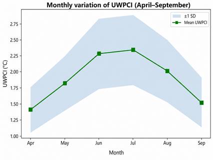
Fig. 6. Monthly variation in UWPCI.
4.1.4 Subregional comparison
The 181 UWPs were divided into three subregions according to their geographical location and natural–socioeconomic conditions: the western gully region (n = 47), central urban agglomeration (n = 78), and southern valley region (n = 56). One-way ANOVA was used to test differences in UWPCI and UWPCE among these subregions.
For UWPCI, the central urban agglomeration had the highest mean value (2.23 ± 0.38 ℃), which was significantly higher than those of the southern valley region (1.79 ± 0.31 ℃) and the western gully region (1.42 ± 0.29 ℃). The ANOVA result was significant (F = 38.6, p < 0.001, η² = 0.42). Tukey’s HSD post hoc test showed that all pairwise differences among the three subregions were significant (p < 0.05).
For UWPCE, the central urban agglomeration (0.36 ± 0.08) and western gully region (0.33 ± 0.08) did not differ significantly (p = 0.12). Both values were significantly higher than that of the southern valley region (0.29 ± 0.07, p < 0.05). This result indicates that although the western gully region had low cooling intensity, its cooling efficiency was not lower than that of the central urban agglomeration. This was mainly because wetlands in the western gully region were generally smaller and more compact.
Global Moran’s I for UWPCI was 0.47 (p < 0.001), indicating significant positive spatial autocorrelation. High-value wetlands tended to be located near other high-value wetlands, while low-value wetlands tended to be located near other low-value wetlands. The LISA cluster map further identified a high–high cluster in the Taiyuan–Jinzhong area and a low–low cluster in Lüliang and western Linfen. These results support the rationale for dividing the study area into the three subregions.
4.2 Relative importance of driving factors
4.2.1 Overall importance
Based on the RF models (n_estimators = 500, max_depth = 10) and SHAP analysis, the mean absolute SHAP values of the 20 candidate driving factors were calculated for UWPCI and UWPCE. After normalization, the relative importance rankings were obtained (Fig. 8).
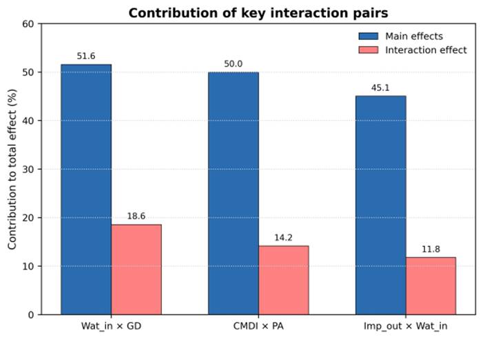
Fig. 7. Subregional comparison of UWP cooling effects.
For UWPCI, the model achieved an R² of 0.76 and an RMSE of 0.21 °C. The dominant factors, with a cumulative contribution greater than 60%, were internal water ratio (Wat_in, 32.7%), gully density (GD, 18.9%), and external impervious surface ratio (Imp_out, 12.4%). The secondary factors were park area (PA, 8.6%), coal-mining disturbance intensity (CMDI, 7.2%), park shape index (PSI, 5.8%), internal vegetation ratio (Veg_in, 4.1%), elevation (Elev, 3.5%), slope (Slope, 2.9%), and external vegetation ratio (Veg_out, 1.9%).
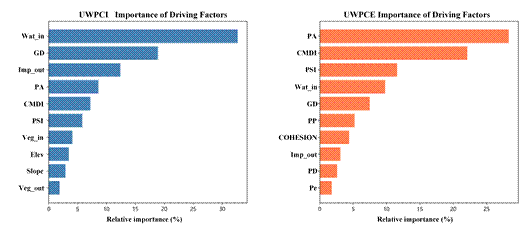
Fig. 8. Relative importance of driving factors.
The combined contribution of the top three factors reached 64.0% (Fig. 9). This indicates that UWP cooling intensity in the Shanxi section was mainly controlled by water availability, terrain fragmentation, and the urban heat island background. Although coal-mining disturbance did not rank among the top three factors, its contribution remained non-negligible.
The combined contribution of PA, CMDI, and PSI was 62.0%. This suggests that cooling efficiency was mainly controlled by the geometric attributes of wetland parks and the disturbance caused by coal mining. The importance of internal water ratio decreased for UWPCE because this index measures cooling capacity per unit area. Excessive water-body allocation may therefore reduce efficiency rather than increase it.
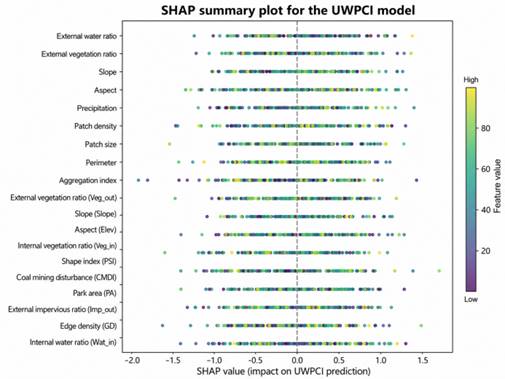
Fig. 9. SHAP summary plot for UWPCI.
The SHAP summary plot further showed the direction of feature effects. High Wat_in values corresponded to positive SHAP values, indicating that a higher internal water ratio increased cooling intensity, although a clear plateau was observed. High GD values corresponded to negative SHAP values, suggesting that stronger terrain fragmentation reduced cooling intensity. The effect of Imp_out was nonlinear. It was positive at low to medium values but became negative at high values.
4.2.2 Subregional differences
Separate RF models were constructed for the three subregions, and the dominant driving factors in each subregion were ranked by relative importance (Fig. 10).
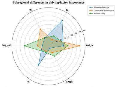
Fig. 10. Radar chart of subregional differences in driving-factor importance.
In the western gully region, the driving-factor priority was GD (34.2%) > CMDI (25.6%) > Wat_in (18.3%). Terrain fragmentation and coal-mining disturbance together contributed nearly 60%, indicating that they were the primary constraints on UWP cooling functions in this subregion. A further comparison showed that wetlands with CMDI > 0.5, mainly located in the Lishi and Liulin mining areas, had UWPCI values 0.61 °C lower than those with CMDI < 0.2 (p < 0.001).
In the central urban agglomeration, the driving-factor priority was Wat_in (38.7%) > Imp_out (22.4%) > PA (14.1%). The urban heat island background, represented by high Imp_out, not only increased cooling demand but also strengthened the cooling benefit of water bodies through heat-island–wetland interactions. This interaction is further examined in Section 4.4.
In the southern valley region, the driving-factor priority was PA (29.8%) > Wat_in (24.1%) > GD (13.2%). Because this subregion has relatively flat terrain, wetland size became the main limiting factor. The importance of internal water ratio was slightly lower than that in the central urban agglomeration but much higher than that in the western gully region.
4.2.3 Model performance and simplified models
For UWPCI, the R² values of the full-factor model and the top-10 model on the validation set were 0.76 and 0.74, respectively. The difference was not significant according to the paired t-test (p = 0.09). Their RMSE values were 0.21 ℃ and 0.22 ℃, respectively, with no significant difference (p = 0.13). For UWPCE, the R² values of the full-factor model and the top-10 model were 0.68 and 0.66, respectively (p = 0.11). Their RMSE values were 0.08 and 0.09, respectively (p = 0.17).
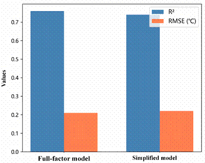
Fig. 11. RF model performance comparison for UWPCI.
These results indicate that the top-10 models retained sufficient predictive accuracy while improving model interpretability. The subsequent analyses therefore used the top-10 simplified models. Residual diagnostics showed that the residuals were approximately normally distributed, with a Shapiro-Wilk test result of p = 0.13 (Fig. 12). The histogram was generally symmetric. No clear trend was observed between residuals and fitted values, and no funnel-shaped or nonlinear pattern appeared. These results indicate that the model did not show evident violations of homoscedasticity.
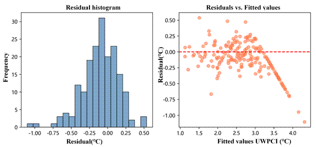
Fig. 12. Residual diagnostics of the RF model.
4.3 Partial dependence relationships and threshold effects
4.3.1 Partial dependence relationships for UWPCI
SHAP dependence plots revealed clear threshold effects for the key driving factors of UWPCI (Fig. 13).
Fig. 13. Partial dependence relationships between core factors and UWPCI.
For Wat_in, the relationship followed an S-shaped increasing pattern, with a threshold of approximately 65%. When Wat_in was below 20%, SHAP values were close to zero or slightly negative. This indicates that wetlands with very limited water bodies had weak cooling functions and relied mainly on vegetation transpiration. In arid regions, however, vegetation is often constrained by summer water stress. When Wat_in ranged from 20% to 65%, SHAP values increased almost linearly with Wat_in. The slope was approximately 0.025 SHAP units per percentage point, suggesting that every 10% increase in internal water ratio increased UWPCI by approximately 0.22 ℃. When Wat_in exceeded 65%, SHAP values entered a plateau phase, and further increases in water area did not produce additional cooling gains. Segmented regression identified the breakpoint at 64.8%, with a 95% confidence interval of 62.3%–67.1%. The Pettitt test confirmed the significance of this change point (p < 0.001).
This pattern indicates that evaporative cooling from water bodies dominates in arid regions. However, after Wat_in exceeds approximately 65%, the marginal cooling contribution of additional water surface declines. This may occur because near-surface humidity approaches saturation and because excessive water area reduces vegetation space, thereby weakening the synergistic role of vegetation transpiration.
For GD, the relationship showed a negative decay pattern, with a threshold of approximately 2.5 km/km². When GD was below 1.5 km/km², SHAP values showed a small positive contribution, ranging from approximately +0.1 to +0.2 ℃. Under this condition, terrain had a limited but positive effect on cold-air accumulation. When GD ranged from 1.5 to 2.5 km/km², SHAP values changed rapidly from positive to negative, and UWPCI decreased from 2.1 ℃ to 1.6 ℃. When GD exceeded 2.5 km/km², SHAP values stabilized at approximately −0.5 ℃, and cooling intensity decreased by about 40%. Excessively developed gullies caused cold air to drain rapidly along valley channels, preventing the wetland cool island from accumulating effectively.
In the western gully region, 34 UWPs had GD values greater than 2.5 km/km². Their mean UWPCI was only 1.28 ℃, which was significantly lower than that of wetlands with GD values below 2.0 km/km² (1.71 ℃; t = 5.23, p < 0.001).
For external impervious surface ratio (Imp_out), the relationship first increased and then decreased, with a peak around 45%. When Imp_out was below 30%, SHAP values were close to zero. Under this condition, the background temperature was not high enough to create a strong temperature contrast, and the cooling benefit of wetland parks was limited. When Imp_out ranged from 30% to 45%, the urban heat island effect intensified, and the wetland–urban temperature contrast increased. SHAP values became significantly positive and reached their maximum at approximately 42%–45%. When Imp_out exceeded 45%, excessive impervious surfaces raised the background temperature and enhanced turbulent heat flux. This exceeded the buffering capacity of wetland evaporative cooling, and the relative cooling benefit began to decline.
This threshold suggests that UWP siting should prioritize areas with moderately high urban heat island intensity, where Imp_out is approximately 35%–45%. These locations can better match cooling demand with wetland cooling capacity, rather than placing wetlands in the most intensely heated urban cores.
4.3.2 Partial dependence relationships for UWPCE
For PA, the relationship with UWPCE followed a logarithmic growth pattern, with an optimal range of 0.9–1.1 km² (Fig. 14a). When PA was below 0.3 km², UWPCE increased rapidly with park area, with a slope of approximately 0.12 per km². Although small wetlands had limited absolute cooling intensity, their cooling area per unit buffer area was high. When PA ranged from 0.5 to 1.5 km², the increase in UWPCE slowed, rising from 0.32 to 0.38. UWPCE reached its highest efficiency range when PA was between 0.9 and 1.1 km², with a peak value of 0.42 ± 0.03. Beyond this range, further increases in park area led to a slow decline in UWPCE. At PA = 2.5 km², UWPCE decreased to 0.35.
This result has direct implications for land-saving wetland planning. In the Shanxi section, simply expanding wetland area does not produce a proportional increase in cooling efficiency and may lead to inefficient land use.
For CMDI, the relationship was linearly negative, with an ineffective threshold of approximately 0.6 (Fig. 14b). When CMDI increased from 0 to 0.3, UWPCE decreased only slightly, from 0.36 to 0.34, suggesting that the wetland could still maintain basic cooling functions. When CMDI ranged from 0.3 to 0.6, UWPCE entered a functional decline stage, decreasing at a rate of approximately −0.04 for every 0.1 increase in CMDI. When CMDI exceeded 0.6, UWPCE dropped sharply below 0.20. The model prediction intervals indicated that wetlands under this level of disturbance had almost lost their ecological cooling function.
Field verification showed that UWPs with CMDI values greater than 0.6 commonly had land-subsidence cracks, with crack density exceeding 0.5 m/m², severe water leakage, with daily leakage exceeding 8 cm, and large-scale dieback of emergent plants.
Fig. 14. Partial dependence relationships between core factors and UWPCE.
4.3.3 Subregional differences in key thresholds
Subregional threshold values differed among the western gully region, central urban agglomeration, and southern valley region (Table 4). For Wat_in, the optimal upper limits were 58%, 68%, and 62%, respectively. In the western gully region, water loss through evaporation was greater, and excessive water-body allocation increased the frequency of shallow-water drying. As a result, the effective water-body proportion was reduced. In the central urban agglomeration, the optimal upper limit was higher because the stronger urban heat island background increased the cooling benefit of water bodies. For PA, the optimal ranges were 1.0–1.3 km² in the western gully region, 0.7–1.0 km² in the central urban agglomeration, and 0.9–1.2 km² in the southern valley region. In the central urban agglomeration, high land cost and strong urban heat island intensity allowed relatively small wetlands to achieve higher cooling efficiency. For Imp_out, the suitable ranges were 30%–40% in the western gully region, 35%–48% in the central urban agglomeration, and 32%–42% in the southern valley region. In the western gully region, the urban heat island effect was weaker, and excessive impervious surface cover was often associated with more severe soil erosion and water loss.
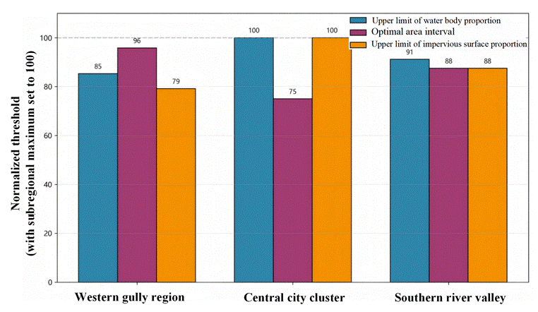
Fig. 15. Subregional comparison of key thresholds.
Table 4. Subregional thresholds of key driving factors.
| Factor | Western gully region | Central urban agglomeration | Southern valley region | Explanation |
| Optimal upper limit of Wat_in (%) | 58 | 68 | 62 | In arid areas, water-body evaporation loss is high. Excessive water-body allocation increases the frequency of shallow-water drying, thereby reducing the actual effective water-body proportion. |
| Optimal range of PA (km²) | 1.0–1.3 | 0.7–1.0 | 0.9–1.2 | In the central urban agglomeration, land cost is high. Small wetlands can achieve relatively high cooling efficiency by benefiting from the urban heat island contrast. |
| Suitable range of Imp_out (%) | 30–40 | 35–48 | 32–42 | In the western gully region, the urban heat island effect is weaker. Excessive impervious surface cover is often accompanied by more severe soil erosion and water loss. |
Threshold validation further confirmed the 65% threshold for Wat_in (Fig. 16). In the below-threshold group, where Wat_in was less than 65%, UWPCI was significantly and positively correlated with Wat_in (r = 0.71, p < 0.001), with a regression slope of 0.023. In the above-threshold group, where Wat_in was at least 65%, this correlation disappeared (r = 0.09, p = 0.42). The dispersion of UWPCI also increased, with the standard deviation rising from 0.31 to 0.48. This indicates that after the optimal water-body ratio is exceeded, other factors, such as water quality and water-exchange frequency, begin to dominate cooling performance.
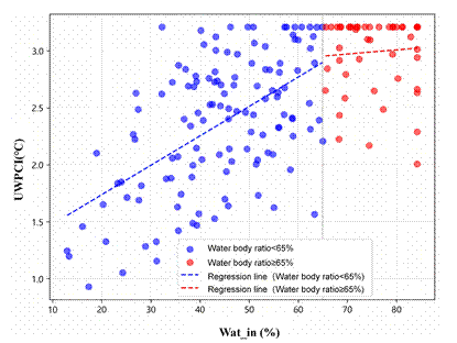
Fig. 16. Validation of the threshold effect of internal water ratio at 65%.
4.4 Interaction effects of driving factors
4.4.1 Key interaction pairs
The SHAP interaction-value matrix and the Geodetector interaction analysis identified three interaction pairs with clear synergistic or antagonistic effects (Fig. 17).
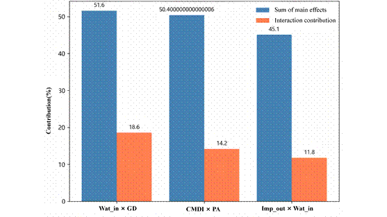
Fig. 17. Contribution ratios of key interaction pairs.
The interaction between Wat_in and GD accounted for 18.6% of the total effect and showed nonlinear enhancement (Fig. 18). The Geodetector results showed that the q value of the Wat_in × GD interaction was 0.67, higher than the q values of the two individual factors. This indicates that water-body configuration and terrain fragmentation jointly shaped the spatial differentiation of UWPCI. The SHAP interaction contour plot further clarified this mechanism. When Wat_in was below 60%, the negative effect of GD was amplified, and the SHAP interaction value reached approximately −0.32. This means that fragmented terrain intensified the cooling disadvantage caused by insufficient water bodies. When Wat_in exceeded 65%, the negative effect of GD on UWPCI was largely offset, and the interaction value approached zero. Sufficient water bodies can therefore partly compensate for fragmented terrain by maintaining local evaporative cooling. A compensatory relationship was also observed along the diagonal direction of the contour plot. For every 0.5 km/km² increase in GD, Wat_in needed to increase by approximately 8%–10% to maintain a similar UWPCI level.
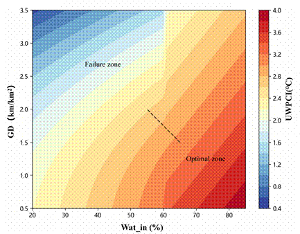
Fig. 18. Interaction contour plot of internal water ratio and gully density.
The interaction between CMDI and PA accounted for 14.2% of the total effect and showed a synergistic weakening pattern. Coal-mining disturbance not only reduced UWPCE directly but also weakened the positive contribution of park area to cooling efficiency. When CMDI was below 0.3, the marginal contribution of PA to UWPCE was +0.18 per km². When CMDI exceeded 0.5, this marginal contribution decreased to +0.06 per km², a reduction of 67%. Mining-induced land subsidence damaged the integrity of wetland boundaries and reduced the effective park area. At the same time, mine pit water is often acidic or highly mineralized, which can inhibit plant growth and weaken evaporation-related cooling.
The interaction between Imp_out and Wat_in accounted for 11.8% of the total effect and showed synergistic enhancement. When Imp_out exceeded 40% and Wat_in exceeded 55%, the SHAP interaction value reached +0.41. This value was 1.7 times the sum of the individual contributions of Wat_in and Imp_out, which were approximately 0.30 and 0.15, respectively. This heat-island–water-body synergy was an important source of high UWPCI in the central urban agglomeration. However, when Imp_out exceeded 55%, the interaction value became negative. This indicates that excessive urbanization can exceed the mitigation capacity of wetland cooling.
4.4.2 Subregional differences in interaction contribution
The interaction-to-main-effect ratio differed markedly among the three subregions (Fig. 19). In the western gully region, the ratio reached 142.6%, meaning that the interaction contribution exceeded the sum of the main effects. This suggests that UWP cooling in this subregion was jointly constrained by multiple pressures. Optimizing a single factor is therefore unlikely to produce a strong cooling improvement. Joint interventions that combine water-body enhancement, terrain restoration, and mining regulation are required. In the central urban agglomeration, the interaction-to-main-effect ratio was 112.8%. Interaction effects were evident, but the main effects remained dominant. Increasing internal water ratio and optimizing the external landscape context can therefore still produce substantial cooling gains. In the southern valley region, the interaction-to-main-effect ratio was 98.3%, close to an additive effect. Interaction effects were relatively weak in this subregion, and the major driving factors can be optimized in a more independent manner.
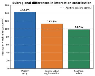
Fig. 19. Subregional differences in interaction contribution ratios.
5 Discussion
5.1 Distinctiveness of UWP cooling effects in the Shanxi section
The mean cooling intensity of UWPs in the Shanxi section of the Yellow River Basin was 1.85℃. This value was lower than those reported for wetlands in the Yangtze River Basin and the Beijing–Tianjin–Hebei region, but slightly higher than that of grassland wetlands in the arid region of Inner Mongolia. The comparison indicates that aridity, fragmented terrain, and coal mining jointly constrain wetland cooling functions in the study area. The arid climate increases water-body evaporation loss. During warm-season afternoons, the relative humidity inside wetlands was only 52%, which weakened the continuity of evapotranspiration cooling. The fragmented terrain of the Loess Plateau restricted horizontal cold-air diffusion, and the cooling effect declined by 63% beyond a distance threshold of 500 m. Coal-mining disturbance further damaged wetland hydrological connectivity. Nearly half of the wetland parks located above mined-out areas experienced seasonal drying.
Reclaimed coal-mining wetlands showed a distinct low-intensity but high-efficiency pattern. Their mean cooling intensity was only 1.34℃, whereas their cooling efficiency reached 0.38. This pattern can be explained by the physical form of reclaimed mining wetlands. Most of them consist of small pond clusters, and their dense edge interfaces support efficient cooling per unit area. This finding offers a planning option for arid and semi-arid regions where water resources are limited.
5.2 Regional specificity of driving mechanisms
The western gully region showed a terrain-mining dual-constraint mechanism. The interaction contribution of gully density and coal-mining disturbance intensity reached 142.6%, indicating that these two factors formed a reinforcing constraint. Coal-mining subsidence intensified terrain fragmentation, while fragmented terrain accelerated soil erosion and water loss in mining areas. In active mining zones, UWP cooling intensity declined at an average rate of 0.12℃ per year. Wetlands in closed mining areas required approximately three to five years before functional recovery began. This suggests that ecological restoration in mining areas should be managed across the full life cycle.
The central urban agglomeration showed a water-body–impervious-surface synergy. The interaction between urban heat island intensity and internal water ratio played a dominant role. When external impervious surface ratio increased from 30% to 45%, the optimal threshold of internal water ratio increased from 58% to 72%. However, the per capita water resources in the Taiyuan Basin are only 173 m³. Expanding water bodies without constraint is therefore not sustainable. Reclaimed-water use is needed to support long-term water-body maintenance.
The southern valley region showed an area-water-body synergy. This subregion has relatively favorable water resources and flat terrain. UWP cooling effects were mainly driven by the linear combination of park area and internal water ratio. When both factors were at medium to high levels, UWPCI exceeded 2.4℃. This provides empirical support for constructing the Baili ecological corridor along the Fenhe River Valley.
5.3 Optimized spatial-layout strategies
Based on the above findings, this study proposes a differentiated strategy centered on zoning-based classification, threshold-based regulation, and mine–wetland coordination.
In the western gully region, a distributed micro-wetland network should be developed. The terrain of coal-mining subsidence areas can be used to construct a multistage pond-ditch-wetland cascade system, with each unit covering 0.05-0.15 km². The spacing between units should be less than 300 m to maintain cool-island connectivity. Ecological buffer zones wider than 50 m should be established to reduce sediment deposition. Full-cycle management should also be implemented, including pre-mining protection, in-mining monitoring, and post-mining restoration.
In the central urban agglomeration, targeted blue–green integration should be promoted. For newly planned wetland parks, the internal water ratio should be controlled within 60%-68% to avoid the diminishing marginal benefit observed beyond approximately 65%. Reclaimed-water replenishment systems should be developed, with a target reclaimed-water utilization rate of at least 40%, to maintain the minimum ecological water level during dry seasons. Wetland layout should also be coupled with urban ventilation corridors. Priority should be given to areas where the external impervious surface ratio is around 40%.
In the southern valley region, large-scale ecological main corridors should be constructed. Existing wetland parks should be connected along the main axis of the Fenhe River to form a continuous cold-source corridor longer than 150 km. The recommended unit area is 0.9–1.1 km². River–wetland hydrological connectivity should be maintained, and the designed ecological baseflow should not be lower than 5 m³/s. Agricultural non-point source pollution control should also be coordinated with wetland planning.
A common support system is also needed across the three subregions. This system should include an integrated satellite–aerial–ground monitoring network, the incorporation of cooling-effect indicators into wetland protection performance assessment, and a public-facing “urban wetland cooling map” mini-program to support public participation.
5.4 Limitations and future research
This study has several data-related limitations. The impervious surface data for 2025 were simulated by extrapolating trends from the GAIA 2020 dataset, which introduces uncertainty. Coal-mining disturbance intensity incorporated mine distribution and production capacity, but local factors such as mining depth and backfilling technology were not considered. The cooling effect was evaluated using warm-season mean LST, and differences between daytime and nighttime cooling were not distinguished.
Several model-related limitations also remain. The black-box nature of RF restricts the explicit representation of some physical mechanisms. Future studies could explore hybrid approaches that combine structural equation modeling with machine learning. The 20 driving factors used in this study may also omit micro-hydrological processes, such as groundwater depth and soil moisture. In addition, the interaction analysis focused only on pairwise interactions. Higher-order interactions involving three or more factors require further investigation.
Future research should focus on three directions. The first is the coupled water-heat-carbon mechanism of wetland cooling in arid regions. The second is the long-term succession of wetland ecological restoration in coal-mining subsidence areas, which would benefit from fixed monitoring plots lasting more than 10 years. The third is the optimal configuration of wetland park networks at the regional scale. This would shift the focus from single-park optimization to the maximization of network-level cooling performance.
6 Conclusions
First, the 181 UWPs in the Shanxi section of the Yellow River Basin had a mean cooling intensity of 1.85 ± 0.42 ℃ and a mean cooling efficiency of 0.31 ± 0.09. These values were lower than those reported for humid regions in China. Spatially, the cooling effect showed a pattern of higher values in the central region and lower values in the western and southern regions. The central urban agglomeration had the highest cooling intensity, with a mean value of 2.23 ℃, whereas the western gully region had the lowest value, at 1.42 ℃. Temporally, July and August were the peak cooling months. During drought years, cooling intensity decreased by more than 20%.
Second, the dominant driving factors of cooling intensity were internal water ratio, with a contribution of 32.7%, gully density, with a contribution of 18.9%, and external impervious surface ratio, with a contribution of 12.4%. The dominant driving factors of cooling efficiency were park area, with a contribution of 28.3%, coal-mining disturbance intensity, with a contribution of 22.1%, and park shape index, with a contribution of 11.6%. These results reveal a distinctive driving pattern shaped by the combined pressures of aridity, fragmented terrain, and coal mining.
Third, several key threshold effects were identified. When the internal water ratio exceeded 65%, the marginal cooling benefit approached zero. When gully density was greater than 2.5 km/km², cooling intensity decreased by 40%. When coal-mining disturbance intensity exceeded 0.6, cooling efficiency was largely lost. Park area reached its optimal cooling efficiency within the range of 0.9–1.1 km².
Fourth, the driving mechanisms differed substantially among subregions. In the western gully region, cooling effects were jointly constrained by terrain fragmentation and coal mining, with an interaction contribution of 142.6%. In the central urban agglomeration, the interaction between internal water ratio and external impervious surface ratio was dominant, and the optimal water-body threshold increased with urban heat island intensity. In the southern valley region, park area and internal water ratio showed a synergistic enhancement pattern. Wat_in × GD, CMDI × PA, and Imp_out × Wat_in were identified as the three key interaction pairs.
Fifth, this study proposes a differentiated optimization strategy centered on zoning-based classification, threshold-based regulation, and mine–wetland coordination. A distributed micro-wetland network is recommended for the western gully region. Targeted blue–green integration should be implemented in the central urban agglomeration. Large-scale ecological main corridors should be developed in the southern valley region. These strategies are aligned with ecological protection in the Yellow River Basin and ecological restoration in coal-mining areas. They provide scientific evidence and technical support for urban wetland planning and heat island mitigation in arid and semi-arid regions.
Funding: This research received no external funding.
Institutional Review Board Statement: N/A.
Informed Consent Statement: N/A.
Data Availability Statement: Data will be available on reasonable request.
Conflicts of Interest: The authors declare no conflicts of interest.
References:
- Xue Y, Ren C, Lau KK-L, et al. Urban wetland parks and their cooling effects on surrounding environments. Ecological Indicators, 2019.
- Deng Y, Jiang W, Yao Y, et al. Analysis of urban wetland park cooling effects and their potential influence factors: Evidence from 477 urban wetland parks in China. Ecological Indicators, 2023, 156:111103.
- Deng Y, Jiang W, Ling Z, et al. Revealing the driving factors of urban wetland park cooling effects using Random Forest regression and SHAP algorithm. Sustainable Cities and Society, 2025, 120:106151.
- Liu L, He H, Cai Y, et al. Cooling effects of wetland parks in hot and humid areas based on remote sensing images and local climate zone scheme. Building and Environment, 2023, 243:110660.
- Yan Y, et al. How do landscape patterns affect cooling intensity and scale? Evidence from 13 primary urban wetlands in China. Ecological Indicators, 2024, 166:112574.
- Ye Y, Qiu H. Urban wetland parks: A systematic review of ecological functions and planning. Land, 2021.
- Zhou W, et al. Urban wetlands and ecosystem services: A review. Ecological Indicators, 2020.
- Mitsch WJ, Gosselink JG. Wetlands. 5th ed. Wiley, 2015.
- Davidson NC. Wetland ecosystem services. Marine and Freshwater Research, 2014.
- Urban Wetlands: A Review on Ecological and Cultural Values. Water, 2021.
- Bowler DE, Buyung-Ali LM, Knight TM, Pullin AS. Urban greening to cool towns and cities. Landscape and Urban Planning, 2010.
- Feyisa GL, Dons K, Meilby H. Efficiency of parks in mitigating urban heat island effect. Landscape and Urban Planning, 2014.
- Lu J, et al. A micro-climatic study on cooling effect of an urban park. Sustainable Cities and Society, 2017.
- Yan H, et al. Influence of a large urban park on the local urban thermal environment. Science of the Total Environment, 2018.
- Xie M, et al. Park cooling island intensity: A review. Urban Forestry & Urban Greening, 2020.
- Sensing-based park cooling performance observation and assessment: A review. Building and Environment, 2023.
- Jiménez-Muñoz JC, et al. Revision of the single-channel algorithm for land surface temperature retrieval. IEEE Transactions on Geoscience and Remote Sensing, 2009.
- Sobrino JA, Jiménez-Muñoz JC, Paolini L. Land surface temperature retrieval from Landsat TM 5. Remote Sensing of Environment, 2004.
- Ermida SL, et al. Google Earth Engine open-source code for land surface temperature estimation from the Landsat series. Remote Sensing, 2020.
- Wulder MA, et al. Current status of Landsat program. Remote Sensing of Environment, 2019.
- Breiman L. Random forests. Machine Learning, 2001.
- Lundberg SM, Lee SI. A unified approach to interpreting model predictions. Advances in Neural Information Processing Systems, 2017.
- Lundberg SM, Erion G, Lee SI. Consistent individualized feature attribution for tree ensembles. Nature Machine Intelligence, 2020.
- Chen J, et al. Quantifying the main and interactive effects of dominant factors on land surface temperature using SHAP. Sustainable Cities and Society, 2024.
- Wang JF, Li XH, Christakos G, et al. Geographical detectors-based health risk assessment. International Journal of Geographical Information Science, 2010.
- Wang JF, Xu CD. Geodetector: Principle and prospective. Acta Geographica Sinica, 2017.
- Fu BJ, Wang S, Liu Y, et al. Ecological restoration in the Loess Plateau. Earth-Science Reviews, 2017.
- Chen YP, et al. Ecological protection and high-quality development of the Yellow River Basin. Journal of Geographical Sciences, 2020.
- Wang J, et al. Coal mining and ecological restoration in China. Journal of Cleaner Production, 2021.
- Ferreira CSS, et al. Soil degradation in the European Mediterranean region: Processes, status and consequences. Science of the Total Environment, 2022.